ICT Optimal Trade Entry, commonly called ICT OTE, is one of the most recognized entry concepts in the ICT (Inner Circle Trader) methodology. Developed and taught by Michael J. Huddleston, this concept is covered in the ICT Forex – Market Maker Primer Course and focuses on entering retracements after a meaningful directional price move.
The concept is simple in principle.
When the market is bullish, the trader looks to buy a retracement after an impulse move higher.
When the market is bearish, the trader looks to sell a retracement after an impulse move lower.
As Michael J. Huddleston explains:
“Optimal trade entry is really based on buying retracements.”
However, ICT Optimal Trade Entry is not simply about drawing a Fibonacci tool on every price swing. The trader first needs directional context, a meaningful price level, institutional sponsorship, and a break in market structure.
What Is ICT Optimal Trade Entry?
ICT Optimal Trade Entry is a retracement-based entry model that attempts to position a trader deep inside a corrective price movement before the market resumes its expected direction.
The basic bullish model is:
Bullish Bias → Impulse Move Higher → Market Structure Break → Retracement → OTE Buy → Expansion Higher
The bearish model is:
Bearish Bias → Impulse Move Lower → Market Structure Break → Retracement → OTE Sell → Expansion Lower
OTE allows the trader to enter during a retracement rather than chasing price after the directional move has already started.
In simple terms:
Bullish Market → Buy the Retracement
Bearish Market → Sell the Rally
The important part is determining which retracement is worth trading.
ICT OTE Starts With Higher Timeframe Context
Before looking for an Optimal Trade Entry, Huddleston emphasizes the importance of higher timeframe price levels.
The trader should study charts such as:
- Monthly
- Weekly
- Daily
- Four-hour
The purpose is to identify areas where price previously moved away aggressively.
For example:
Price Reaches Higher Timeframe Resistance → Strong Sell-Off
This can indicate institutional selling interest.
Similarly:
Price Reaches Higher Timeframe Support → Strong Rally
This can indicate institutional buying interest.
Huddleston explains that the trader is looking for:
“Evidence that there’s going to be an institutional sponsorship behind the price move.”
OTE should therefore be connected to a broader directional narrative.
Random Fibonacci retracements on lower timeframes do not automatically create valid ICT Optimal Trade Entries.
Identify Important Higher Timeframe Levels
ICT teaches traders to simplify higher timeframe analysis.
An important level can be as simple as:
- An old monthly high
- An old monthly low
- An old weekly high
- An old weekly low
- An important daily level
The trader studies whether price has previously shown sensitivity around that level.
Suppose price trades above an old monthly high.
The old high may now become an important reference level for potential support.
Once a key higher timeframe level is established, the trader can move to lower timeframes and wait for evidence that price is ready to expand in the expected direction.
The sequence becomes:
Higher Timeframe Level → Institutional Reaction → Market Structure Shift → Retracement → OTE
Market Structure Break Is Important for ICT OTE
A valid ICT Optimal Trade Entry should generally follow an impulse move that breaks market structure.
Suppose price is expected to move higher.
Price rallies and breaks above a meaningful short-term or intermediate-term high.
This shows willingness to deliver higher prices.
The structure is:
Higher Timeframe Support → Bullish Reaction → Swing High Broken
After the high is broken, price may retrace lower.
This retracement creates the potential OTE buying opportunity.
Huddleston explains:
“That impulse price move has to be incorporating a break in market structure.”
The bearish model is reversed.
Higher Timeframe Resistance → Bearish Reaction → Swing Low Broken → Retracement Higher → OTE Sell
Without the market structure break, the retracement may simply be part of an existing opposing trend.
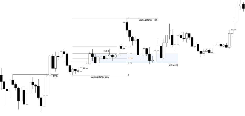
Bullish ICT Optimal Trade Entry
A bullish ICT OTE setup begins with a bullish directional expectation.
Price then produces an impulse move higher and breaks a significant swing high.
The trader identifies the price leg from the impulse low to the impulse high.
The Fibonacci retracement tool is applied to this price leg.
The process is:
Impulse Low → Impulse High → Fibonacci Retracement
The trader then waits for price to retrace into the Optimal Trade Entry area.
The bullish framework is:
Bullish Bias → Market Structure Break Higher → Retracement Into OTE → Buy → Target Higher Prices
The objective is to buy the retracement before the next expansion higher.
Bearish ICT Optimal Trade Entry
The bearish ICT Optimal Trade Entry uses the opposite structure.
Price produces an impulse move lower and breaks an important swing low.
The Fibonacci retracement tool is drawn from the impulse high to the impulse low.
The sequence becomes:
Impulse High → Impulse Low → Fibonacci Retracement
The trader then waits for price to retrace higher into the OTE area.
The bearish model is:
Bearish Bias → Market Structure Break Lower → Retracement Into OTE → Sell → Target Lower Prices
The trader is effectively selling the rally rather than chasing the original bearish impulse.
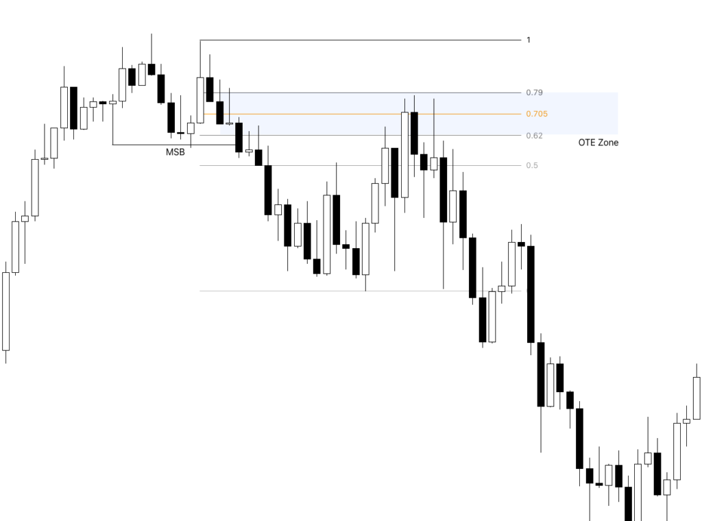
ICT OTE Fibonacci Levels
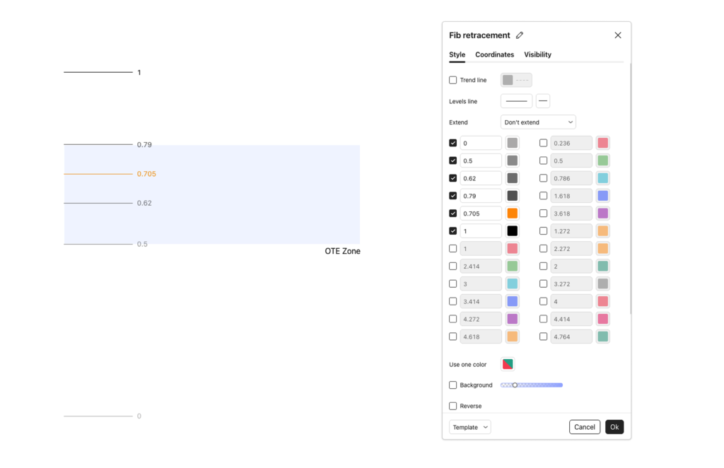
The ICT Optimal Trade Entry zone is generally framed between the 62% and 79% Fibonacci retracement levels.
The primary retracement levels discussed in the model are:
- 62%
- 70.5%
- 79%
Huddleston describes 70.5% as the preferred sweet spot.
He explains:
“It’s 0.705 for the sweet spot for optimal trade entry.”
Therefore, the OTE zone can be viewed as:
62% Retracement → Beginning of OTE Area
70.5% Retracement → OTE Sweet Spot
79% Retracement → Deeper OTE Limit
The trader does not always need price to reach exactly 70.5%.
Price may react from any point inside the broader 62% to 79% retracement range.
The 70.5% OTE Sweet Spot
The 70.5% retracement level is commonly associated with ICT Optimal Trade Entry.
It represents a deep retracement into the previous impulse move.
The advantage of entering deeper into the retracement is improved trade location.
For example, in bullish conditions:
Impulse Move Higher → Price Retraces Deeply → Entry Near 70.5% → Stop Near Impulse Low → Higher Upside Objective
A deeper entry may reduce the distance between entry and invalidation.
This can improve the reward-to-risk profile.
However, traders should not force the 70.5% level.
Huddleston notes that he may seek a fill closer to the 62% retracement rather than demanding the deepest possible entry.
The OTE zone is a framework, not a requirement that price touch one exact number.
Drawing Fibonacci on Candle Bodies
An important detail in the ICT OTE approach is how the price swing is measured.
Huddleston emphasizes studying the bodies of the candles.
For a bullish impulse, the Fibonacci tool may be anchored from the relevant body low to the highest open or close of the impulse swing.
For a bearish impulse, the opposite measurement is used.
The reasoning is that candle wicks can vary between brokers and price feeds.
Huddleston states:
“We want to look at the price move on the bodies of the candles.”
This method attempts to reduce the influence of inconsistent wick pricing.
The focus is on the core price delivery represented by the candle bodies.
OTE Is Not a Supply and Demand Zone
ICT Optimal Trade Entry should not be confused with a generic supply and demand zone.
A broad zone-based trader may identify an area and assume price can react anywhere inside it.
ICT OTE uses specific Fibonacci retracement levels within a defined impulse price leg.
The process is structured:
Identify Direction
Identify Structural Break
Measure Impulse Swing
Define 62%–79% Retracement
Wait for Price to Reach the OTE Area
The objective is to narrow the potential entry location rather than mark a large undefined zone.
Bullish OTE Example
Suppose price is trading near an important higher timeframe support level.
Price reacts higher and breaks a short-term high.
A second, more significant intermediate-term high is also broken.
This provides stronger bullish structural confirmation.
The trader measures the bullish impulse leg.
Price then retraces into the 62% to 79% area.
The setup becomes:
Higher Timeframe Support → Bullish Market Structure Break → OTE Retracement → Long Entry
The stop is positioned around the impulse low or logical invalidation point.
The trader then targets higher liquidity.
Bearish OTE Example
Suppose price reaches an important higher timeframe resistance level.
Price rejects and breaks below a meaningful swing low.
This creates a bearish impulse leg.
The trader measures the price move from the impulse high to the impulse low.
Price then retraces higher into the OTE zone.
The sequence becomes:
Higher Timeframe Resistance → Bearish Market Structure Break → OTE Retracement → Short Entry
The stop is positioned around the impulse high or structural invalidation point.
The trader targets lower liquidity or another logical downside objective.
OTE Stop-Loss Placement
Huddleston teaches that risk should be defined before the trade is entered.
In a bullish OTE setup, the stop may be placed at the relevant impulse low.
For bearish conditions, the stop may be positioned at the impulse high.
The bullish framework is:
Impulse Low → Stop-Loss
OTE Retracement → Entry
Higher Prices → Profit Objectives
The bearish framework is:
Impulse High → Stop-Loss
OTE Retracement → Entry
Lower Prices → Profit Objectives
The distance between the entry and invalidation level defines the trade risk.
The trader should then adjust position size according to the percentage of account equity they are willing to risk.
First Profit and Scaling in ICT OTE
An important part of the ICT Optimal Trade Entry model is knowing where to take profits.
For a bullish trade, the old impulse high becomes an important first reference point.
For a bearish trade, the old impulse low becomes the equivalent level.
However, Huddleston prefers taking some profit slightly before the old high or low because price can fail to trade through it.
He explains:
“At that high or just below it, that’s where my first profit is.”
This first profit is more accurately described as the first scaling point.
It allows the trader to reduce exposure before price reaches the larger expansion targets.
ICT OTE Fibonacci Profit Targets
The Fibonacci framework also includes expansion levels for profit objectives.
Common levels discussed in the model include:
- 0 level
- -0.27 extension
- -0.62 extension
- -1.00 symmetrical price swing
The first reference level is around the previous impulse high or low.
Additional objectives are based on Fibonacci extensions.
For bullish conditions:
OTE Buy → Old High → 1.27-Type Extension → 1.62-Type Extension → Symmetrical Price Swing
For bearish conditions:
OTE Sell → Old Low → Lower Extension → Deeper Extension → Symmetrical Price Swing
The exact objective depends on the trader’s broader directional bias.
What Is a Symmetrical Price Swing?
A symmetrical price swing is a measured move where the next price expansion is equal in range to the original impulse leg.
Suppose the bullish impulse moves 100 pips.
A symmetrical price swing projects another 100-pip move from the relevant reference point.
The idea is:
Original Impulse Range = Projected Expansion Range
Huddleston describes this as:
“A perfectly symmetrical price swing.”
Price does not always reach the full measured move.
This is why partial profit-taking and scaling are included in the model.
ICT OTE and Reward-to-Risk
Huddleston places significant emphasis on the reward available at the first scaling objective.
He does not simply calculate theoretical reward by projecting an extremely distant target.
The trader should evaluate whether the first reasonable profit area provides sufficient compensation for the risk.
Huddleston explains:
“It needs to be enough of the position coming off that promotes at least two to one.”
The preferred structure is approximately:
Risk = 1R
First Meaningful Profit = Approximately 2R
This does not mean every trade will produce exactly a 2:1 reward-to-risk ratio.
However, the entry should generally provide enough room to justify the risk.
Why a Deep OTE Entry Improves Risk-to-Reward
The deeper the entry inside the retracement, the closer the trader may be to the logical invalidation level.
For example:
Shallow Entry → Wider Stop Distance → Lower Reward-to-Risk
Deep OTE Entry → Smaller Stop Distance → Same Target → Better Reward-to-Risk
This is one reason the 70.5% level is preferred.
Huddleston explains:
“That’s why I want to get as deep as I can into that 70.5 level.”
However, waiting for the deepest retracement can also result in missed trades.
The trader must balance entry quality with realistic execution.
Institutional Price Levels and OTE
The OTE model can also be combined with institutional price levels.
Huddleston discusses price increments such as:
- Full figures
- 20 levels
- 50 levels
- 80 levels
For example:
1.1700 → Full Figure
1.1720 → Institutional Level
1.1750 → Mid Figure
1.1780 → Institutional Level
1.1800 → Next Full Figure
When an OTE retracement aligns with one of these algorithmic price levels, the confluence may strengthen the setup.
The process can appear as:
Higher Timeframe Level → Institutional Price Level → Market Structure Break → OTE Retracement
The trader is combining price location with retracement structure.
ICT OTE and Liquidity
Liquidity plays an important role in determining profit objectives.
Suppose a bullish OTE forms.
The trader should look above current price.
Where are the old highs?
Where might buy stops be resting?
The market may seek those buy stops as price expands higher.
The bullish sequence becomes:
Institutional Buying → OTE Retracement → Reaccumulation → Expansion Higher → Buy-Side Liquidity
For bearish trades:
Institutional Selling → OTE Retracement → Redistribution → Expansion Lower → Sell-Side Liquidity
Liquidity provides a logical reason for the market to move toward the target.
Lower Timeframe OTE vs Higher Timeframe OTE
OTE can appear on multiple timeframes.
However, Huddleston cautions against becoming overly focused on very low timeframes.
A one-minute or five-minute OTE may have a very small price range.
An hourly setup may provide a larger directional opportunity and more room for favorable reward-to-risk.
The larger framework should therefore begin with higher timeframe analysis.
A practical approach is:
Monthly/Weekly/Daily Context → 4H or 1H Structure → 15-Minute Entry Refinement
Lower timeframes can refine execution, but they should not replace the broader narrative.
ICT OTE and the Market Maker Buy Model
A bullish Optimal Trade Entry can appear during the reaccumulation phase of an ICT Market Maker Buy Model.
The sequence may look like:
Consolidation → Price Moves Away → Return to Consolidation → Smart Money Reversal → Low-Risk Buy → Reaccumulation → Expansion
An OTE can form during the reaccumulation stage.
Price breaks market structure higher.
The retracement allows additional buying before price expands into higher liquidity.
The bearish version can appear during redistribution inside a Market Maker Sell Model.
A Simple ICT Optimal Trade Entry Process
Step 1: Start With Higher Timeframe Analysis
Study monthly, weekly, and daily price levels.
Step 2: Determine Bullish or Bearish Conditions
Identify whether price is expected to move higher or lower.
Step 3: Wait for an Impulse Move
Price should move strongly in the expected direction.
Step 4: Confirm Market Structure Break
Bullish setups should break an important high.
Bearish setups should break an important low.
Step 5: Measure the Impulse Leg
Use the Fibonacci retracement tool on the relevant price swing.
Step 6: Mark the OTE Zone
Identify the 62% to 79% retracement area.
Pay particular attention to the 70.5% level.
Step 7: Wait for the Retracement
Do not chase the original impulse move.
Step 8: Define Risk
Use the relevant structural high or low as the invalidation point.
Step 9: Identify First Scaling
Look near the previous impulse high or low.
Step 10: Identify Expansion Targets
Use liquidity and Fibonacci extension levels.
The complete process is:
Higher Timeframe Narrative → Market Structure Break → Impulse Swing → OTE Retracement → Entry → Scaling → Liquidity Target
Common Mistakes When Trading ICT OTE
Drawing Fibonacci on Every Swing
Not every price swing creates a valid ICT Optimal Trade Entry.
There should be directional context and a meaningful structural break.
Ignoring Higher Timeframe Levels
OTE is stronger when connected to institutional higher timeframe price levels.
Chasing the Impulse Move
The model is based on waiting for a retracement.
Buying the high of a bullish impulse defeats the purpose of OTE.
Demanding the Exact 70.5% Level
Price can react anywhere within the broader OTE zone.
The 70.5% level is a preferred sweet spot, not a guaranteed turning point.
Ignoring Risk Before Entry
The invalidation level and position size should be determined before executing the trade.
Using a Distant Target to Create Fake Reward-to-Risk
The first realistic scaling objective should provide sufficient room to justify the trade risk.
Final Thoughts
ICT Optimal Trade Entry is a retracement-based entry model designed to help traders participate in directional price movement from a favorable price location.
The core bullish model is:
Bullish Higher Timeframe Context → Market Structure Break Higher → Retracement Into 62%–79% OTE → Buy → Target Buy-Side Liquidity
The bearish model is:
Bearish Higher Timeframe Context → Market Structure Break Lower → Retracement Into 62%–79% OTE → Sell → Target Sell-Side Liquidity
The 70.5% retracement is commonly treated as the OTE sweet spot, but the setup is not created by Fibonacci alone.
A valid ICT OTE requires context.
Higher timeframe price levels provide the narrative. Market structure provides confirmation. The impulse swing defines the retracement. Fibonacci provides a framework for entry. Liquidity and expansion objectives define the potential targets.
The real purpose of Optimal Trade Entry is not to predict every market turn. It is to wait for the market to show directional intent and then seek a favorable retracement before the next expected price expansion.